
Based on the dynamic DEA model, this paper employs an enhanced common frontier dynamic super-efficiency SBM model to quantitatively evaluate the agricultural carbon emission efficiency of urban agglomerations and their constituent cities. Additionally, spatial pattern evolution analysis is conducted using ArcGIS 10.8 after classification, followed by a comprehensive analysis of the joint threshold requirements for agricultural carbon emission efficiency of urban agglomerations at different levels. Lastly, wave convergence curves are fitted. The basic flowchart of applied methodology is shown in Fig. 1.
Fig. 1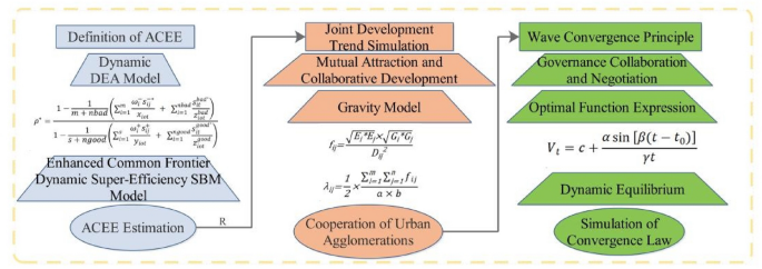
The basic flowchart of applied methodology.
Calculate the agricultural carbon emission efficiency
Initially, this paper develops a dynamic DEA framework, categorizing carryover variables into four kinds including good, bad, free and fixed. It constructs independent decision-making units (DMUs), denoted as \(\left(j=1, 2, \dots ,n\right)\), over T periods \(\left(T=1, 2, \dots , T\right)\), each characterized by multiple unique inputs and outputs, where carryover from period T to T + 1 is formalized in Eq. (1).
$$\mathop \sum \limits_{j = 1}^{n} z_{ijt}^{\alpha } \lambda_{j}^{t} = \mathop \sum \limits_{j = 1}^{n} z_{ijt}^{\alpha } \lambda_{j}^{t + 1} \left( {\forall ;t = 1, \ldots , T – 1} \right)$$
(1)
where, α signifies the kind of variable, encompassing aforementioned variables.
The non-oriented total efficiency \(\left({\delta }^{*}\right)\) is determined via formula (2), \({\omega }^{t}\) and \({\omega }_{i}\) represent the weights assigned to the output and input elements, respectively.
$${\delta }^{*}=\frac{\frac{1}{T}\sum_{t=1}^{T}{\omega }^{t}\left[1-\frac{1}{m+nbad}\left(\sum_{i=1}^{m}\frac{{\omega }_{i}^{-}{s}_{ij}^{-}}{{x}_{iot}} + {\sum }_{i=1}^{nbad}\frac{{s}_{it}^{bad}}{{z}_{iot}^{bad}}\right)\right]}{\frac{1}{T}\sum_{t=1}^{T}{\omega }^{t}\left[1-\frac{1}{s+ngood}\left(\sum_{i=1}^{s}\frac{{\omega }_{i}^{+}{s}_{ij}^{+}}{{y}_{iot}} + {\sum }_{i=1}^{ngood}\frac{{s}_{it}^{good}}{{z}_{iot}^{good}}\right)\right]}$$
(2)
The efficiency of each non-oriented indicator \(\left({\rho }^{*}\right)\) is delineated subsequently.
$${\rho }^{*}=\frac{1-\frac{1}{m+nbad}\left(\sum_{i=1}^{m}\frac{{\omega }_{i}^{-}{s}_{ij}^{-*}}{{x}_{iot}} + {\sum }_{i=1}^{nbad}\frac{{s}_{it}^{{bad}^{*}}}{{z}_{iot}^{bad}}\right)}{1-\frac{1}{s+ngood}\left(\sum_{i=1}^{s}\frac{{\omega }_{i}^{+}{s}_{ij}^{+}}{{y}_{iot}} + {\sum }_{i=1}^{ngood}\frac{{s}_{it}^{{good}^{*}}}{{z}_{iot}^{good}}\right)}$$
(3)
Building on this dynamic DEA model, the study introduces an enhanced common frontier dynamic super-efficiency SBM model, aimed at assessing the agricultural carbon rebound effect. Considering diverse factors, it posits that all units \(\left(N\right)\) consist of \({DMU}_{s}\) organized into multiple groups \(\left(N=N1+N2+\dots +NG\right)\). Here, \({x}_{ij}\) and \({y}_{rj}\) represent the input and output for item \(\text{j}\left(\text{j}=1, 2, \dots ,\text{ N}\right)\) under the common frontier, respectively. Each DMU k is capable of selecting the most favorable output weights to maximize efficiency. The Metafrontier Technical Efficiency of a DMU is then computed utilizing Eq. (4).
$$\text{Min}:{\uprho }^{*}$$
$$\text{s}.\text{t}. {\sum }_{\text{g}=1}^{\text{G}}{\sum }_{\text{j}=1,\text{j}\ne \text{k}}^{\text{n}}{\text{Z}}_{\text{ijtg}}{\uplambda }_{\text{jg}}^{\text{t}}={\sum }_{\text{g}=1}^{\text{G}}{\sum }_{\text{j}=1,\text{j}\ne \text{k}}^{\text{n}}{\text{Z}}_{\text{ijtg}}{\uplambda }_{\text{jg}}^{\text{t}=1}\left(\text{vi}|\text{ t}=1, \dots \text{i}-1\right)$$
$${X}_{iot}={\sum }_{\text{g}=1}^{\text{G}}{\sum }_{\text{j}=1,\text{j}\ne \text{k}}^{\text{n}}{\text{x}}_{\text{ijtg}}{\uplambda }_{\text{jg}}^{\text{t}}+{\text{S}}_{\text{it}}\left(\text{i}=1, \dots ,\text{m};\text{ t}=1, \dots ,\text{ i}\right)$$
$${Y}_{lot}={\sum }_{\text{g}=1}^{\text{G}}{\sum }_{\text{l}=1,\text{l}\ne \text{k}}^{\text{sl}}{\text{y}}_{\text{lot}}^{+\text{g}}{\uplambda }_{\text{j}}^{\text{t}}-{\text{S}}_{\text{lt}}^{+\text{g}}\left(\text{l}=1,\dots ,\text{sl};\text{t}=1,\dots ,\text{T}\right)$$
$${Z}_{iot}^{good}={\sum }_{\text{g}=1}^{\text{G}}{\sum }_{\text{j}=1,\text{j}\ne \text{k}}^{\text{n}}{\text{z}}_{\text{ijtg}}^{\text{good}}{\uplambda }_{\text{jg}}^{\text{t}}-{\text{S}}_{\text{lt}}^{\text{t}}\left(\text{i}=1,\dots ,\text{ngood};\text{t}=1,\dots ,\text{i}\right)$$
$${\sum }_{\text{g}=1}^{\text{G}}{\sum }_{\text{j}=1,\text{j}\ne \text{k}}^{\text{n}}{\uplambda }_{\text{jg}}^{\text{t}}=1\left(\text{t}=1,\dots ,\text{i}\right)$$
$${\uplambda }_{\text{jg}}^{\text{t}}\ge 0,{\text{s}}_{\text{it}}^{-}\ge 0,{\text{s}}_{\text{it}}^{+}\ge 0,{\text{s}}_{\text{it}}^{\text{good}}\ge 0$$
(4)
Joint development trend simulation
The concept of joint intensity encapsulates the magnitude of mutual attraction and collaborative development among cities. Within urban agglomerations, the joint intensity of agricultural carbon emissions is found to be positively associated with the socioeconomic status of the region and inversely related to the geographical distance between cities. As urban agglomerations evolve, shifts in the joint intensity of agricultural carbon emission can serve as a visual representation of the progression in inter-city collaborative development.
This study employs a gravity model to construct a quantitative framework for evaluating the joint intensity of inter-city agricultural carbon emissions within urban agglomerations. The gravity model, traditionally used in physics to describe the attraction between bodies based on mass and distance, is adapted here to measure the “attraction” between cities based on their economic output and geographical proximity. This adaptation allows for an analytical evaluation of how the joint intensity of agricultural carbon emissions changes in response to urban agglomeration dynamics. The mathematical expression of the model is as follows:
$${\text{f}}_{\text{ij}}=\frac{\sqrt{{\text{E}}_{\text{i}}*{\text{E}}_{\text{j}}}\times \sqrt{{\text{G}}_{\text{i}}*{\text{G}}_{\text{j}}}}{{{\text{D}}_{\text{ij}}}^{2}}$$
(5)
where \({\text{f}}_{\text{ij}}\) represents the joint intensity of agricultural carbon emission between cities i and j; \({\text{E}}_{\text{i}}\), \({\text{E}}_{\text{j}}\) signify the agricultural carbon emission efficiency of cities i and j, respectively; \({\text{G}}_{\text{i}}\), \({\text{G}}_{\text{j}}\) signify the GDP of cities i and j, respectively; \({\text{D}}_{\text{ij}}\) represents the square of the distance between cities i and j.
The joint threshold denotes the critical value at which cities commence the division of labor and cooperation to optimize agricultural carbon emission configurations. Although the central city has the need and drive to develop jointly with surrounding cities, due to limitations such as economic ties and geographical distance, the central city can’t unite indefinitely with nearby cities. Thus, there is an objective joint threshold value for agricultural carbon emissions between the central city and nearby cities to determine whether the central city will optimize agricultural carbon emissions jointly with newly integrated cities during a specific period. This study adopts the setting method of previous research23 to reveal the process of optimizing agricultural carbon emissions jointly between the central city and nearby cities. The relevant equation is as follows:
$${\lambda }_{\text{ij}}=\frac{1}{{2}}\times \frac{\sum_{\text{i=1}}^{\text{m}}\sum_{\text{j=1}}^{\text{n}}{f}_{ij}}{a\times b}$$
(6)
where λij signifies the joint threshold value between cities within the urban agglomeration; a signifies the amount of evaluation years; b signifies the amount of cities within the urban agglomeration.
Wave convergence principleTheoretical mechanism
As China’s economic development transitions from rapid growth to high-quality development, profound changes are occurring in the spatial structure, with urban agglomerations becoming critical spatial entities24. The “14th Five-Year Plan” of China has proposed integrated and coordinated development mechanisms for urban agglomerations, and mechanisms for cost-sharing and benefit-sharing, are particularly crucial. Cross-regional coordinated governance of urban agglomerations becomes an inevitable choice, where central cities have the need and motivation to collaborate with surrounding cities to optimize agricultural carbon emission efficiency via the flow of production factors. Drawing on the innovation-led effects and radiating driving effects of urban agglomerations, this paper proposes that during their formation and development, urban agglomerations continually expand their scope and gradually acquire the capacity for joint development. However, inherent resource disparities can easily trap the urban agglomeration carbon systems in a state of resistance23, particularly as inter-city environmental governance collaboration and negotiation during risk-sharing processes may lead to a continuous decrease in carbon emission efficiency. With the persistent improvement of close and effective cooperative relationships, urban agglomerations gradually form an integrated coordinated development entity. The carbon system gradually evolves to an appropriate state where carbon emission efficiency stabilizes at a certain value, as detailed in Fig. 2.
Fig. 2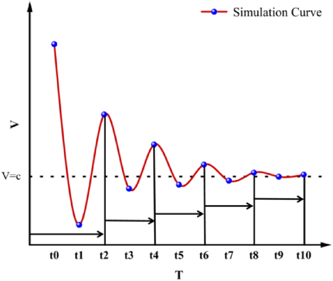
Evolutionary patterns of agricultural carbon emission efficiency in urban agglomerations.
Specifically, in the initial stages of formation, central cities, to maintain their economic growth and environmental quality, often relocate high carbon-emitting industries such as agriculture to smaller surrounding cities. Due to these cities’ lack of technical and managerial capacity to handle increased environmental pressures, such moves, although beneficial to the environmental improvement of central cities in the short term, may lead to an initial drop in efficiency for the entire urban agglomeration. As environmental pressures increase, surrounding cities gradually realize the need for a more equitable distribution of environmental responsibilities and stronger economic compensation, triggering negotiations between cities. Since cities may prioritize protecting their interests over seeking optimal regional collaborative solutions, difficulties in reaching effective agreements may lead to delays in policy implementation, inefficiencies in resource allocation, and inadequate enforcement of environmental measures. Additionally, the decline in carbon emission efficiency may be exacerbated by a lack of long-term perspectives on coordination and sharing, and the absence of effective internal communication and cooperation mechanisms can also lead to a continual decline in overall efficiency. After a period of adjustment and negotiation, as technological advancements and management experience accumulate, the agricultural carbon emission efficiency within urban agglomerations begins to improve and eventually stabilizes at a relatively lower stable value. This stable value not only reflects technological and managerial maturity but also the effectiveness of inter-city collaborative governance, indicating the dynamic equilibrium between regional environmental policies and economic growth.
In the dynamic adjustment of urban agglomeration integration, the heterogeneity in the paths and effects of adaptive adjustments due to inter-group resource differences becomes evident25. Specifically, when new cities unite with central cities and integrate into the development of the urban agglomeration, high antagonism due to differences in population structure, infrastructure, and other factors, may lead to a temporary fall in overall agricultural carbon emission efficiency of the urban agglomeration during this phase. As central cities continue to share their risks with surrounding cities, differences in environmental responsibilities, economic benefits, and resource allocation among cities trigger inter-city environmental collaborative governance and negotiations, further contributing to a descend in regional overall agricultural carbon emission efficiency. After continuous adjustments, the urban agglomeration completes its adaptive adjustment and gradually stabilizes, at which point the cities coordinate development. Thus, as time progresses, central cities continuously engage in joint agricultural carbon emission endeavors with surrounding cities, and as new cities continuously integrate into the urban agglomeration, the agricultural carbon emission efficiency in urban agglomerations exhibits a “wave-like convergence” pattern, characterized by periodic fluctuations due to continuous union with surrounding cities. While central cities have the need and motivation to jointly develop with surrounding cities, economic linkages and geographical distances impose constraints, and there are objectively existing threshold values and limits to union intensity, determining whether central cities engage in joint agricultural carbon emission utilization with newly integrated cities during specific periods.
Overall, studying the evolutionary patterns and wave convergence processes of agricultural carbon emission efficiency in urban agglomerations is of significant importance for addressing real-world issues such as “how to achieve continuous low-carbon development of urban agglomeration agriculture,” “how central cities in urban agglomerations unite with surrounding cities to optimize resource allocation and technology application,” and “how the internal agricultural ecosystem of urban agglomerations can operate efficiently and stably.” It is essential to thoroughly assess the characteristics and developmental stages of cities at varying levels and to formulate corresponding policy recommendations. These policies should aim to promote coordinated regional governance and sustainable agricultural practices.
Function model
The evolutionary pattern of agricultural carbon emission efficiency refers to a nonlinear composite change curve formed over time and with the increasing number of joint cities in a time series, which is also known as the urban agglomeration agricultural carbon emission efficiency wave convergence curve. The detailed function is represented mathematically as follows:
$${V}_{t}=c+\frac{\alpha \text{sin}\left(\beta t\right)}{\gamma t}$$
(7)
here, \({V}_{t}\) represents the agricultural carbon emission efficiency of the urban agglomeration at time t; c represents the final stable value of the urban agglomeration agricultural carbon emission efficiency; Δt is the period of function fluctuation, and Δt = π/β is the amplitude of the trigonometric function, representing the resistance coefficient of the urban agglomeration agricultural carbon emission efficiency; \(\beta\) indicates the periodic coefficient of the urban agglomeration agricultural carbon emission efficiency, with \(\uppi /\upbeta\) being the frequency of the trigonometric function. To enhance the accuracy of the mathematical model, it is optimized. Initial time \({t}_{0}\) and initial value \({V}_{0}\) are assigned to the core city, representing the original time and the original efficiency of the urban agglomeration agricultural carbon emission, respectively. The optimized function curve simulation formula is as follows:
$${V}_{t}=\left\{\begin{array}{c}{V}_{{t}_{0}}={V}_{0},t={t}_{0}\\ c+\frac{\alpha \text{sin}\left[\beta (t-{t}_{0})\right]}{\gamma t},t>{t}_{0}\end{array}\right.$$
(8)
$$\text{X}={\text{x}}_{\text{ij}}\left({\text{t}}_{\text{k}}\right),\text{i}=\text{1,2},\dots ,\text{m};\text{j}=\text{1,2},\dots ,\text{n};\text{k}=\text{1,2},\dots ,\text{K}$$
(9)
When \(\left(n-1\right)\times \frac{\pi }{\beta }, it indicates that the core city in the urban agglomeration collaborates with the n + 1-th city for joint development, and there is a noticeable antagonistic effect in the urban joint development. When \(\left(n-1\right)\times \frac{\pi }{\beta }+\frac{{\text{sin}}^{-1}\frac{\gamma t\left({V}_{t}-c\right)}{\alpha }}{\beta }, it suggests that the core city in the urban agglomeration collaborates with n cities for joint development, leading to a synergistic development effect. The corresponding quantitative analysis is illustrated in Fig. 3.
Fig. 3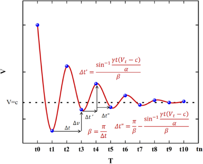
Quantitative analysis of agricultural carbon emission efficiency curves in urban agglomerations.
Index construction
Urban agglomerations are regions formed by the interconnection and collaboration of multiple cities, and it is of great necessity to consider the effect of individual city agricultural carbon emission efficiencies on the efficiency of the urban agglomeration, reflecting the essence of it as a “group” of cities. Therefore, the efficiency level of the urban agglomeration is calculated by averaging the agricultural carbon emission efficiencies of selected cities within the agglomeration. The following detailed indicators are selected to evaluate the agricultural carbon emission efficiency:
Input Indicators: Essential elements are selected from three aspects of the urban agricultural carbon emission system: land, labor, and capital. Land, as the basic resource for agricultural production, is directly related to the potential scale of output, soil carbon storage, and land management practices. Considering the differences in the multiple cropping index and the impact of fallowing in some regions, the total sown area of grain crops (\({10}^{3}{\text{mh}}^{2}\)) is employed to measure land input. To reflect the labor intensity of agricultural production on carbon emissions, labor input is evaluated by the number of people employed in the primary sector (\({10}^{4}\) people). Considering the general state of agricultural production, capital input is examined in four areas: pesticide and fertilizer usage, agricultural machinery, agricultural electricity consumption, and effective irrigation area. The actual amounts of pesticides and fertilizers used (\({10}^{4}t\)), agricultural electricity consumption (\({10}^{4}kw/h\)), and effective irrigation area (\({10}^{3}{\text{mh}}^{2}\)) are based on the actual consumption in the agricultural production process in each region; agricultural machinery input is measured by the total rated power of agricultural machinery used in that year (\({10}^{4}\) kw), including all equipment used for basic agricultural construction, crop transportation, and initial processing of agricultural products.
Output Indicators: ① Expected Output Indicator: To reflect the overall economic benefit of agricultural activities, as well as the overall efficiency and outcomes of agricultural production, the total output value of agriculture, forestry, animal husbandry, and fishery of each city (\({10}^{8}\) yuan) is used as the proxy variable. ② Unexpected Output Indicator: Agricultural carbon emissions serve as an intuitional measure of the environmental impact of agricultural production, which is vital for modern agriculture aiming to achieve ecological efficiency. The agricultural carbon emissions of each city (\({10}^{4}\) t) serve as a proxy variable for unexpected output. Given the current reality of lacking statistical data on it, this article follows the approach21 to examine agricultural carbon emissions from the following angles: inputs of agricultural materials, rice cultivation, and livestock breeding. The specific calculation formula is as follows:
$$\text{C}=\sum {\text{C}}_{\text{i}}=\sum {\text{T}}_{\text{i}}\times {\updelta }_{\text{i}}$$
(10)
The C denote the total agricultural carbon emissions, and \({\text{C}}_{\text{i}}\) represent the emissions from various carbon sources. Variables \({\text{T}}_{\text{i}}\) and \({\updelta }_{\text{i}}\) correspond to the quantity of each carbon source and its respective emission coefficient, respectively. Agricultural inputs primarily include production materials such as chemical fertilizers, pesticides, agricultural plastic films, and diesel fuel, as well as production activities like agricultural irrigation. Rice cultivation encompasses various categories, including early-season, mid-season, and late-season rice. Livestock and poultry breeding covers the main domesticated species. In addition to carbon dioxide emissions, the estimation also incorporates methane (\({CH}_{4}\)) and nitrous oxide (\({N}_{2}O\)) emissions. To facilitate unified analysis, all greenhouse gas emissions are converted into standard carbon equivalents referring to the IPCC Fourth Assessment Report.
Specific indicators corresponding to each category are listed in Table 1.
Table 1 Index selection for the agricultural carbon emission efficiency.
The descriptive statistics are provided in Table 2.
Table 2 Descriptive statistics of the selected indicators.Data sources
Considering the official urban agglomeration development planning documents, the study area primarily encompasses five major national-level urban agglomerations focused on key construction—Yangtze River Delta (YRD), Pearl River Delta (PRD), Beijing-Tianjin-Hebei (BTH), Middle Reaches of Yangtze River (MRYR), Chengdu-Chongqing (CC); eight steadily constructed Regional-level urban agglomerations—Central and Southern Liaoning (CSL), Shandong Peninsula (SP), West Bank of the Strait (WBS), Harbin and Changchun (HC), Central Plains (CP), Guanzhong Plain (GP), Beibu Gulf (BG), the Northern Slope of Tianshan Mountains (NSTM); and six guided and nurtured Provincial-level urban agglomerations—Jinzhong (JZ), Hohhot-Baotou-Ordos-Yulin (HBOY), Central Yunnan (CY), Central Guizhou (CG), Lanzhou-Xining (LX), Along the Yellow River in Ningxia (AYRN), totaling nineteen urban agglomerations. Upon excluding cities with incomplete data, the ultimate sample interval selected for this research encompasses data from 189 cities, as concretely depicted in Fig. 4.
Fig. 4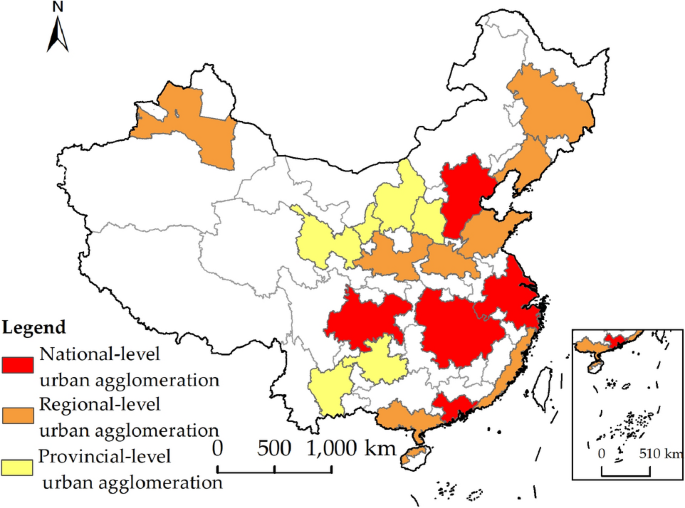
The distribution map of urban agglomerations in China.
The data sources for this study are divided into two parts: 1. Geographic Information Base Data. The National Geomatics Center of China (http://www.ngcc.cn/) released China’s 1:1,000,000 base geographic information data in 2020, which serves as the source for vector administrative boundary maps. Utilizing ArcGIS 10.8 software, urban agglomeration boundaries were merged according to administrative boundary maps to create vector maps of urban agglomerations. 2. Economic and Social Factual Data. The National Economic and Social Development Statistical Bulletins from 2003 to 2021, along with resources including the China Urban Construction Yearbook, China City Statistics Yearbook, and China Urban Agriculture Statistics Yearbook, provided the socio-economic data used in this study. Missing data were imputed using a moving average interpolation technique.